In 2006, Hinton’s Science paper “Reducing the Dimensionality of Data with Neural Networks” presented the Autoencoder (AE), a neural network architecture designed to compress high-dimensional data into a compact latent representation before reconstructing the original input. This approach demonstrated superior performance compared to both Principal Component Analysis (PCA) and its nonlinear variant, Kernel PCA.
Training deep networks was unsolved back then, requiring Hinton to use layer-by-layer pretraining with Restricted Boltzmann Machines (RBMs) for his 9-layer autoencoder. Pascal Vincent’s 2008 Stacked Denoising Autoencoders improved on RBMs for initialization, but researchers eventually discovered that simple random initialization worked equally well, making these pretraining methods obsolete.
This blog post takes you on a journey forward from the autoencoder’s inception, tracing how this foundational idea evolved into today’s flourishing generative AI landscape. I’ll explore my hypothesis that the autoencoder provides a unified conceptual framework for understanding the evolution of VAEs, Diffusion Models, and Flow Matching.
Now imagine you’re a researcher in 2006 who decides to reproduce Hinton’s experiment after reading his science paper. You have access to modern tools—PyTorch, AdamW, GPU acceleration—but you’re constrained by 2006’s conceptual understanding of what’s possible.
Step 1: Reproducing Hinton’s Autoencoder (code)
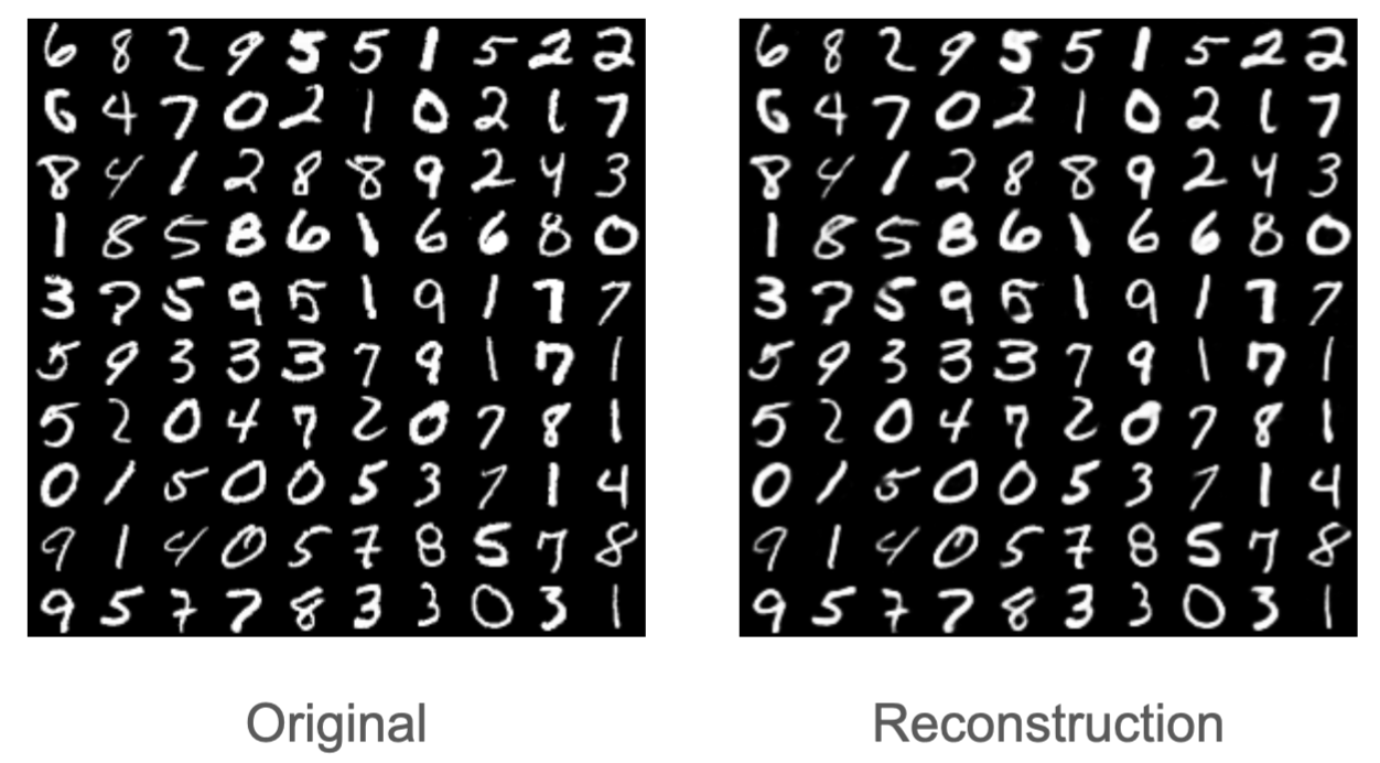
Hinton’s autoencoder has nine layers: 784-1000-500-250-30-250-500-1000-784 neurons, matching MNIST’s 28×28 pixel dimensions at input and output. Using sigmoid activations, MSE loss, and standard optimizations (AdamW, learning rate warmup, gradient clipping), your model achieved a test loss of 3.36 after being trained for 100 epochs on a modest Nvidia 3060 GPU in one minute—close to Hinton’s 3.00 and far better than kernel PCA’s 8.01. The reconstructions are nearly perfect, making further optimization unnecessary.
Notably, your model compresses the original 784-dimensional input into just 30 dimensions. These 30-dimensional latent variables (denoted as $z$) function like biological DNA, capturing nearly all essential image information in a compact representation.
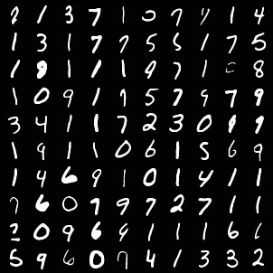
Below are examples comparing original images (left) with their reconstructions (right):
Step 2: Conceptual Breakthrough—Generating Novel Images
You study the reconstructed images, recognizing both progress and limitation. Yes, the system generates images—but only by reproducing what it’s already seen. Real breakthrough would mean creating entirely new images that never existed in the training data. That kind of generative power would reveal true understanding of what makes an image, echoing Feynman’s insight: “What I cannot create, I do not understand.”
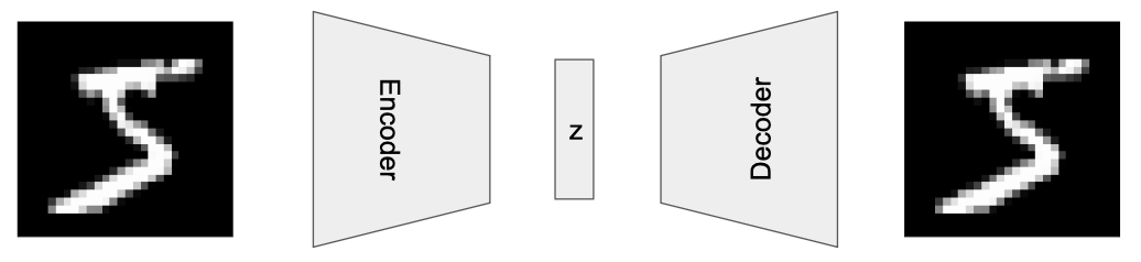
You examine the encoder-decoder architecture carefully. The encoder is familiar—it’s the standard approach for classification tasks, the bread and butter of discriminative AI. But the decoder is where things get interesting: it takes a compact 30-dimensional latent vector $z$ and reconstructs it back into a full image.
Step 3: Exploring the Latent Space (code)
You decide to experiment: what happens when the 30-dimensional vector is slightly modified? What if small amounts of noise are added—say, 0.1 times normal distribution noise? Well, the generated image remains virtually identical to the input.
Next, you try zeroing out the final few dimensions. The generated image still closely resembles the original.
This behavior is expected due to the local continuity of the learned image manifold in latent space.
Out of curiosity, you input random noise and discover that the resulting output image is nearly unrecognizable.
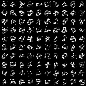
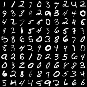
Step 4: Gaussian Mixture Modeling (code)
You sink into deeper contemplation. The key is choosing an appropriate prior distribution for the latent space—one that can be fit to the observed samples. The natural choice emerges: a Gaussian Mixture Model (GMM).
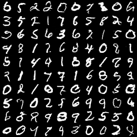
Using standard tools like sklearn’s GaussianMixture, you fit a GMM to the encoder’s latent vectors from the training data. Sampling from this fitted distribution and passing the samples through the decoder produces new images below.
The theory works! You’ve generated genuinely new images that never existed in the training set. Despite their imperfections, these digits confirm you’re on the right path forward.
Step 5: Toward Variational Autoencoder (code)
Before celebrating, you pause. This approach can’t learn online—it requires offline preprocessing to fit the Gaussian mixture model.
The solution: build an autoencoder where the latent code must both reconstruct images and conform to a known distribution. Once trained, generate images by sampling from that distribution. The challenge: how do you constrain latent features to follow a specific distribution, such as a Gaussian?
This demands abandoning deterministic thinking and reimagining the problem probabilistically. You realize that the latent variable $z$ is fundamentally a random variable, not a fixed point. What $z$ “should be” is inherently uncertain—even its dimensionality is ambiguous. If 30 dimensions reconstruct images successfully, wouldn’t 40 also suffice? Clearly yes. Even fixing 30 dimensions, small perturbations to $z$ barely affect reconstruction quality. Thus $z$ isn’t a point—it’s a probability distribution, analogous to an electron’s quantum wavefunction: a cloud of possibility.
A traditional autoencoder optimizes $z$ to minimize reconstruction error, but now the objective is different: sample $z$ from a Gaussian distribution and have it successfully restore the original image. However, when $z$ comes from random sampling rather than the encoder’s output, the backpropagation chain breaks. You can’t take derivatives through a random number generator, so the encoder receives no gradient updates.
After much deliberation, the solution arrives like a midnight revelation—the Reparameterization Trick: a Gaussian random variable can be expressed as a function of a standard normal variable $\epsilon \sim \mathcal{N}(0,1)$, namely $z=\mu + \sigma \times \epsilon$, where $\mu$ and $\sigma$ are the mean and standard deviation respectively. In the forward process, the encoder outputs $\mu$ and $\sigma$, while simultaneously sampling from $\epsilon$ to generate $z$ for the decoder. In the backward process, the reconstruction error gradient flows back to the encoder through $\mu$ and $\sigma$.
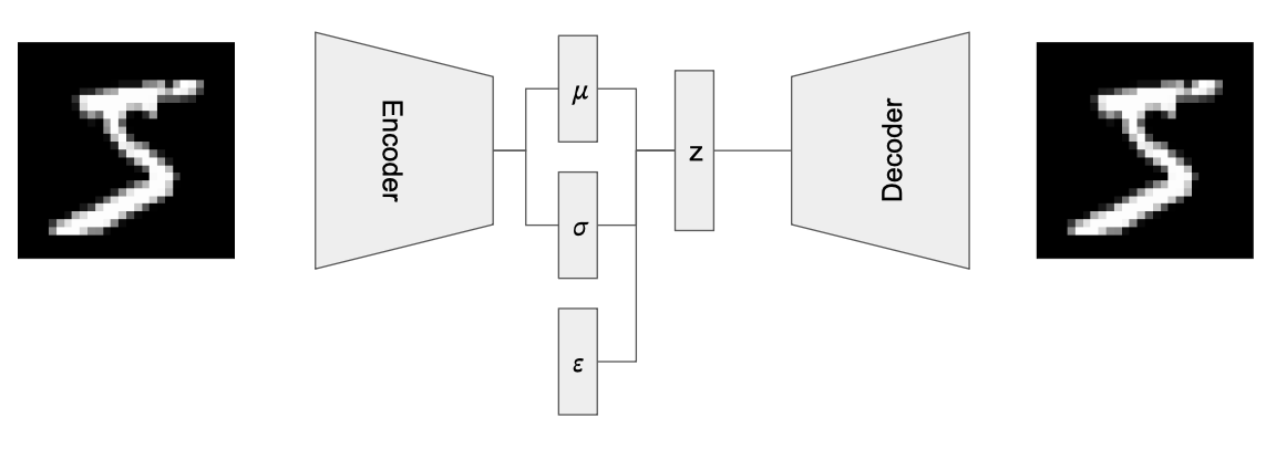
But this alone is insufficient. The variable $z$ must be constrained to follow a standard normal distribution. How should similarity between two probability distributions be measured? KL divergence is the answer. After some derivation, you find that the following term must be added to the loss function:
$$\frac{1}{2}(\mu^2 + \sigma^2 - \log(\sigma^2) - 1)$$
This creates a multi-objective optimization problem—minimize both reconstruction error and the KL divergence between $z$ and the standard normal distribution. Careful adjustment of the two objectives’ weights ensures the gradients they produce remain balanced, with neither overwhelming the other.
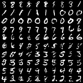
After training completes, you sample from the standard normal distribution and feed the samples to the decoder:
Brand new images emerge—data generated by an end-to-end online learning algorithm, simple and elegant. A deep sense of satisfaction washes over you, an indescribable feeling of achievement.
Step 6: Questioning and Reflection
For a while, satisfaction reigns. You share the method with colleagues, proud of the elegant solution. The work feels complete—time to move on.
Then reality intrudes. A colleague mentions casually: the generated images appear somewhat blurry. Others voice concerns: the weight balancing reconstruction and KL divergence proves exceptionally difficult to tune—a finicky hyperparameter that dramatically impacts results.
Step 7: Toward Diffusion Models (code)
You find yourself thinking deeply again.
Returning to first principles, you begin to question: wasn’t our original intention simply to transition one probability distribution into another? Why must we obsess over the information compression part (that $z$ vector)? Why can’t we directly generate images from random noise? Yes, why not?
You immediately conduct a simple experiment: have the autoencoder directly predict images from input random noise, using MSE between predicted and real images as the loss function.
The output is extremely blurry—the network has only learned what an “average” digit looks like. Generating clear images from random noise in a single step is too hard.
Then inspiration strikes! You remember the Denoising Autoencoder from earlier: it could easily reconstruct images from slightly corrupted versions—can this idea be generalized? You grab some paper and sketch out a process:
Original image → Light corruption → Medium corruption → Heavy corruption → Complete noise
If the network can recover from light noise, why not from medium to light noise? Or even from complete noise to heavy noise? The insight is clear: break the impossible leap from noise to image into many small, learnable steps.
The next question is: how do you design this learning path? How do you gradually add noise to images? You realize this requires support from mathematical tools. Ready for some symbols and formulas? Don’t worry, I promise to use only the most necessary ones.
Forward Process: Adding Noise
Let $x_0$ be the original image, and $x_t(0 \le t \le T, t \in \mathbb{Z})$ denote the image obtained after applying $t$ noise addition operations. Assume each addition is Gaussian noise $\mathcal{N}(0, \beta_t)$, where $0 \lt \beta \lt 1$ controls noise intensity. To ensure image variance remains stable after continuous noise addition, the original image needs to be scaled to $\sqrt{1-\beta_t}$ times. Given $x_{t-1}$, the distribution of $x_t$ can be expressed as:
\[q(x_t|x_{t-1}) = \mathcal{N}(x_t; \sqrt{1-\beta_t}x_{t-1}, \beta_t I) \tag{1}\]
To simplify derivation, let $\alpha_t = 1-\beta_t$ and $\bar{\alpha}_t = \prod^{t}_{1} \alpha_t$. Use $\epsilon$ to represent a standard normal distribution random variable. Equation (1) can be rewritten as1:
$$ \begin{aligned} x_t & = \sqrt{{\alpha}_t} x_{t-1} + \sqrt{1-{\alpha}_t} \epsilon_{t-1} \\ & = \sqrt{{\alpha}_t}(\sqrt{{\alpha}_{t-1}}x_{t-2} + \sqrt{1-{\alpha}_{t-1}}\epsilon_{t-2}) + \sqrt{1-{\alpha}_t}\epsilon_{t-1} & \text{\small expand } x_{t-1}\\ & = \sqrt{{\alpha}_t {\alpha}_{t-1}}x_{t-2} + \sqrt{{\alpha}_t(1-{\alpha}_{t-1})}\epsilon_{t-2} + \sqrt{1-{\alpha}_t}\epsilon_{t-1} & \text{ \small } \\ & = \sqrt{{\alpha}_t {\alpha}_{t-1}}x_{t-2} + \sqrt{1-{\alpha}_t{\alpha}_{t-1}}\tilde{\epsilon}_{t-2} & \text{\small Note 1 } \\ & = … \\ & = \sqrt{\bar{\alpha}_t} x_0 + \sqrt{1 - \bar{\alpha}_t} \epsilon \tag{2} \end{aligned} $$
(Note 1): $\epsilon_{t-1}$ and $\epsilon_{t-2}$ are two independent random variable that follows standard Gaussian distribution. When they are superimposed, the result is still a Gaussian distribution. The mean of the new distribution is the sum of the original means, and the variance is the sum of the original variances. Therefore, the new variance is: ${\bar{\alpha}_t(1-\bar{\alpha}_{t-1}) + {1-\bar{\alpha}_t = 1-\bar{\alpha}_t\bar{\alpha}_{t-1}}}$.
Equation (2) provides a shortcut to obtain $x_t$ directly from $x_0$. Similarly, for $x_{t-1}$:
\[ x_{t-1} = \sqrt{{\bar{\alpha}_ {t-1}}} x_0 + \sqrt{1 - \bar{\alpha}_{t-1}} \epsilon \tag{3}\]
Reverse Process: Recovering Images from Noise
At this point, the forward process (adding noise to images) is clear. Next comes the core challenge—the reverse process: recovering images from noise. You need to calculate the distribution of $x_{t-1}$ given $x_t$. You stare at equations (2) and (3) repeatedly, discovering they share two common variables: $x_0$ and $\epsilon$. Solving them simultaneously and eliminating one variable will greatly simplify the formula.
Both elimination methods are mathematically equivalent; here we use eliminating $x_0$ as an example. From equation (2), it holds that:
$$x_0 = \frac{1}{\bar{\alpha}_t} (x_t - \sqrt{1-\bar{\alpha}_t}\epsilon)$$
Substituting into equation (3) and simplifying:
$$x_{t-1} = \frac{\bar{\alpha}_{t-1}}{\bar{\alpha}_t}(x_t - \sqrt{1-\bar{\alpha}_t}\epsilon) + \sqrt{1-\bar{\alpha} _{t-1}}\epsilon \tag{4}$$
Now $x_{t-1}$ is expressed as a function of $x_t$ and $\epsilon$2. If we can know the specific value of the random variable $\epsilon$, everything will fall into place. You find the last piece of the puzzle: use a neural network with parameters $\theta$ to learn $\epsilon$! That is, optimize the loss function: ${\Vert \epsilon - \epsilon_{\theta}(x_t, t) \Vert_2}$.
Training and Sampling
Everything becomes clear. During training, the network predicts $\epsilon_\theta$ from $x_t$ and $t$; during sampling, substitute $x_t$ and $\epsilon_\theta$ into equation (4), iterating step by step from $t = T, T-1, …, 1$ until obtaining the final image $x_0$.
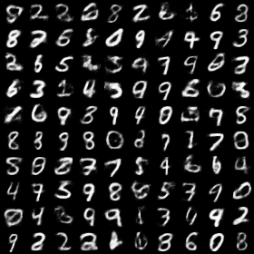
You code this up excitedly. The loss decreases but plateaus, and the images stay blurry. Something’s wrong, you panic a little bit. After reviewing the code, you realize the MLP isn’t powerful enough—you need an architecture built for images. Thinking of image-to-image tasks like segmentation, UNet comes to mind: a fully convolutional encoder-decoder structure that downsamples then upsamples.
You swap in UNet and rerun the code. When clear digit images appear on screen, you know you’ve succeeded. You call it a “Diffusion Model”: like ink diffusing into water, you add noise to images, then use the network to predict and remove it, recovering the originals.
Step 8: Flow Matching—A More Direct Path (code)
You look at the images you’ve generated, impressed by the rigorous mathematical framework behind them. But something nags at you—a feeling you can’t quite put into words.
Then it hits you: you’ve lost your intuition. Somewhere in all those complex formulas, the simple understanding you used to rely on got buried. So you go back to basics and ask yourself: is there an even simpler way to get from noise to image?
The answer comes to you suddenly—a straight line. Just draw a straight line from noise to image using linear interpolation. Why not take the shortest path?
$$ x_t = t x_1 + (1-t) x_0 $$
You dive into experimenting right away. Each round, you randomly pick a value for t (between 0 and 1), feed in $x_t$, and have the network predict $x_0 - x_1$ (the velocity field). You realize you don’t need to be stuck on the autoencoder idea that the output has to be $x_{t-1}$—if predicting the forward direction is more stable, why not just do that?
For sampling, you start with $x_1$ (pure noise) and predict $x_0 - x_1$ at each step. But instead of jumping all the way there, you take a small step, then predict $x_0 - x_1$ again from this new position. You keep doing this until you reach $x_0$ (the real image).
You tweak a few lines in your diffusion code and hit run. The loss keeps dropping—that’s promising! You check the output samples and—it works! This straightforward approach actually works. Without realizing it, you’ve just invented flow matching.
Conclusion: Trust Your Intuition
You’ve traveled from autoencoders to VAEs, from diffusion models to flow matching—and throughout this journey, your skipped the mathematical deep end. Instead, you started with simple, powerful intuitions. Every breakthrough came from asking the right questions: What are you actually trying to do? Is there an easier way?
That’s the approach I want to share: don’t let the math scare you. Build your intuition first. Understand what the problem is really about, then find the simplest solution. Einstein put it well: “If you can’t explain it simply, you don’t understand it well enough.”
The generative AI revolution is here, and it all traces back to that humble autoencoder.