A Tale of Two Fields: On the Emergence of Early Visual Neurons

TLDR: Hubel and Wiesel’s Nobel Prize-winning discoveries ¹ about early visual neurons — cells that respond selectively to center-surround and orientation patterns — sparked decades of computational modeling. Neuroscientists built models (Linsker’s model²³⁴, ICA⁵, Foldiak’s model⁶, and sparse coding⁷) around Hebbian learning⁸ rules that give rise to these same feature-selective representations from raw, unlabeled input. Remarkably, deep neural networks⁹, built by ML/AI researchers and trained with backpropagation¹⁰, arrive at the same representations – a convergence between two fields that have otherwise grown far apart.

It is fascinating and deeply puzzling that the brain, sitting in a dark skull, can form a vivid picture of the outside world by analysing billions of noisy, spiking neurons. Although much remains unknown after decades of research, we at least have a clear understanding of how the early visual system works, thanks to Hubel and Wiesel’s phenomenal work done in the 1960s and 70s.

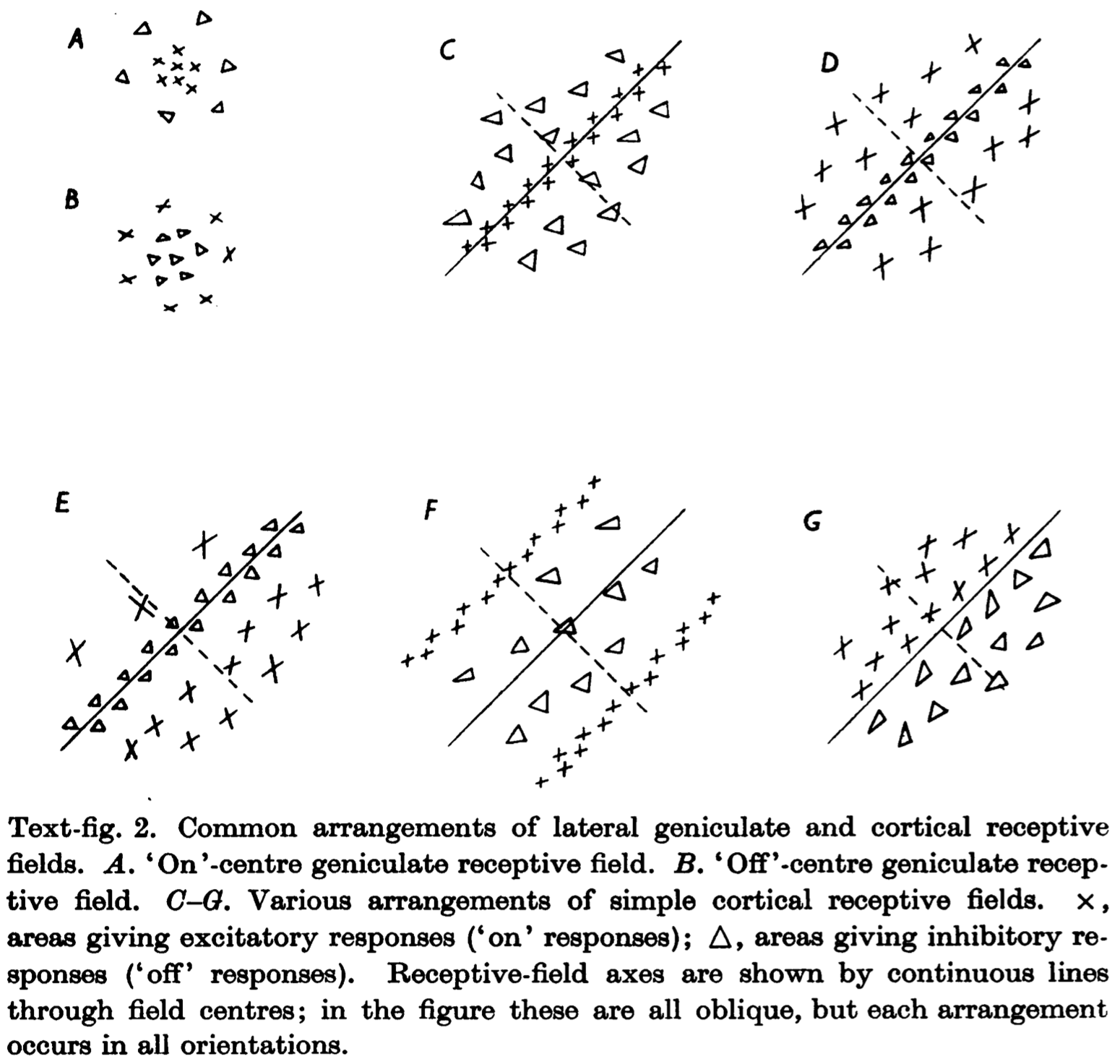
This post focuses on simple-cell receptive fields, some of which are shown below. On/off center cells (A and B) respond best to light or dark stimuli in a spatially-selective area. Orientation-selective cells (C–G) respond best to edges of a particular orientation.

How does the brain construct feature-selective neurons without being explicitly instructed to do so? Are these neurons innate, or are they learned? I proceed from the assumption that at least these neurons can be learned. So what kind of learning rule does the brain follow?

Hebbian Rule

In his landmark 1949 book “The Organization of Behavior”, Hebb offers the following postulate, known as the Hebbian rule:

“When an axon of cell A is near enough to excite a cell B and repeatedly or persistently takes part in firing it, some growth process or metabolic change takes place in one or both cells such that A’s efficiency, as one of the cells firing B, is increased.”

Mathematically speaking, the weight $w_i$ changes in propotional to the correlation between its input $x_i$ and output $y$:

$$\Delta w_i \propto x_i y \tag{1}$$

Linsker’s Model

In a three-paper series published in 1986, Linsker showed that with a Hebbian-style learning rule, a linear neural network with random inputs can develop neurons that are spatially and orientation-selective.

His network comprises 3–4 layers. Each cell in an upper layer connects to $N$ cells in the layer below, randomly selected according to a Gaussian probability distribution (with standard deviation $\sigma$) over distance. Learning is unsupervised: after random initialization, weights are updated layer by layer from low to high for a fixed number of iterations, according to the following partial differential equation:

$$\dot{c} = \sum_j Q_{ij} c_j + k_1 + \frac{k_2}{N} \sum_j c_j$$

where $c$ is the weight vector and $Q$ is the input covariance matrix. The first term is derived from equation $(1)$. Because Hebbian learning leads to unbounded weight growth, $c$ is clipped to the range [−1, 1]. $k_1$ and $k_2$ are hyperparameters.

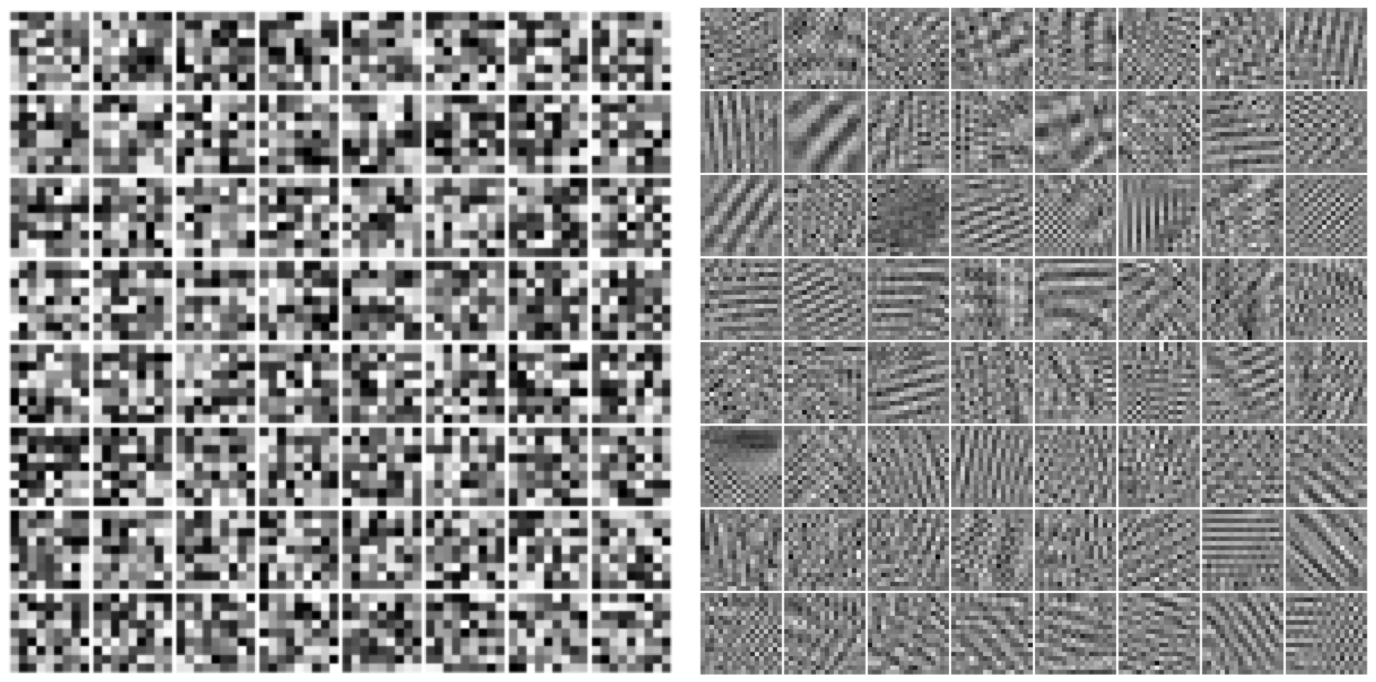
My implementation of Linsker’s model reproduces his findings. The two figures below visualized the receptive fields of spatially-selective cells and orientationally-selective cells separately. To obtain these results, the hyperparameters $\sigma$, $k_1$, and $k_2$ need to be carefully tuned.

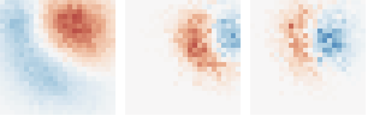
These cells are spatially selective.

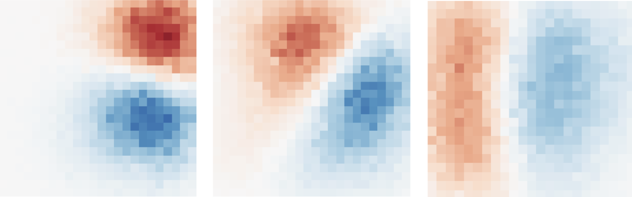
These cells are orientaionally selective.

Hebbian Rule, Variance, PCA, and Mutual Information

Hebbian learning on a single neuron effectively maximizes its output variance. Intuitively, a neuron is uninformative if its output stays constant across inputs; it is most useful and sensative when its output spans a wide dynamic range. (For a more rigorous treatment, see Linsker 1992 paper¹¹ and Olshausen’s lecture notes¹².)

Recall that PCA finds a set of orthogonal bases, each capturing the maximum residual variance. In the special case of weight normalization (Oja’s rule¹³), the output converges to the first principal component of the input.

Under certain conditions — specifically, Gaussian noise — maximizing output variance is equivalent to maximizing its Shannon entropy and, ultimately, mutual information between input and output. Linsker termed this the infomax principle: neurons implicitly learn to transmit as much information as possible. This information-theoretic connection deepens our understanding of Hebbian learning and inspired new models.

ICA

ICA (Independent Component Analysis) builds on the same mutual information maximization principle, but extends it to nonlinear (logistic) neural networks. Formally speaking, mutual information is expressed as:

$$I(X, Y) = H(Y) - H(Y|X)$$

where $X$, and $Y$ are input and output respectively. $H(Y)$ is the output entropy and $H(Y|X)$ measures the uncertainty of $Y$ given $X$. Because the network is deterministic, $Y$ is fully determined by $X$, so $H(Y|X) \approx − \infty$. Maximizing $I(X, Y)$ reduces to maximizing $H(Y)$. After careful calculation, the ICA weight update rule is:

$$\Delta w \propto \frac{1}{w} + x(1 - 2y)$$

It contains an anti-Hebbian term, $-2xy$, that drives weights toward zero and an anti-decay term $\frac{1}{w}$ that penalizes excessively small weights.

ICA can also be understood through the lens of Barlow’s redundancy reduction principle: $H(Y) = \sum_i H(y_i) - H(y_1, y_2, \ldots)$. Maximizing $H(Y)$ requires minimizing $H(y_1, y_2, \ldots)$ — that is, minimizing the shared information across output units — thereby encouraging independence and reducing redundancy.

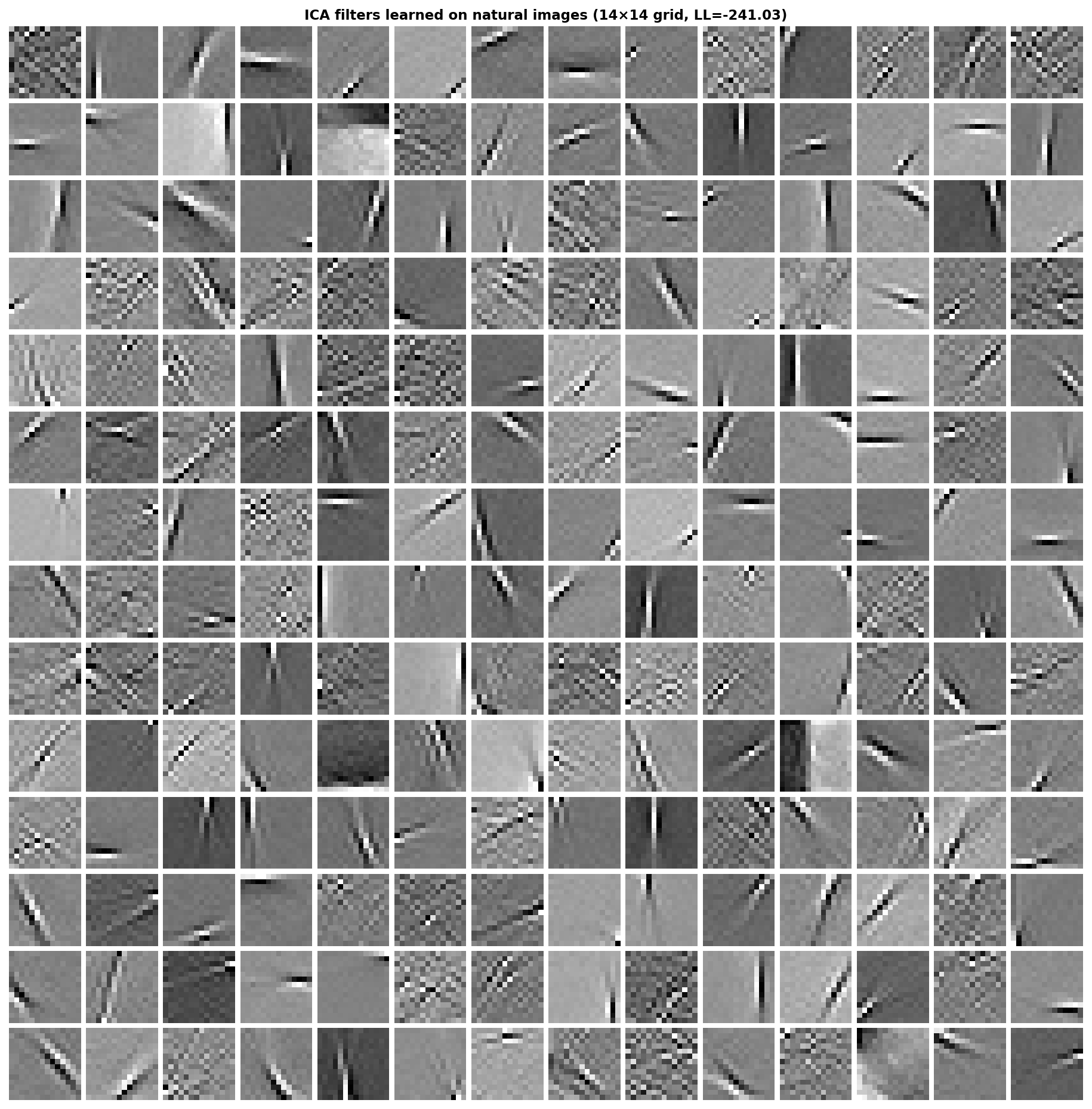
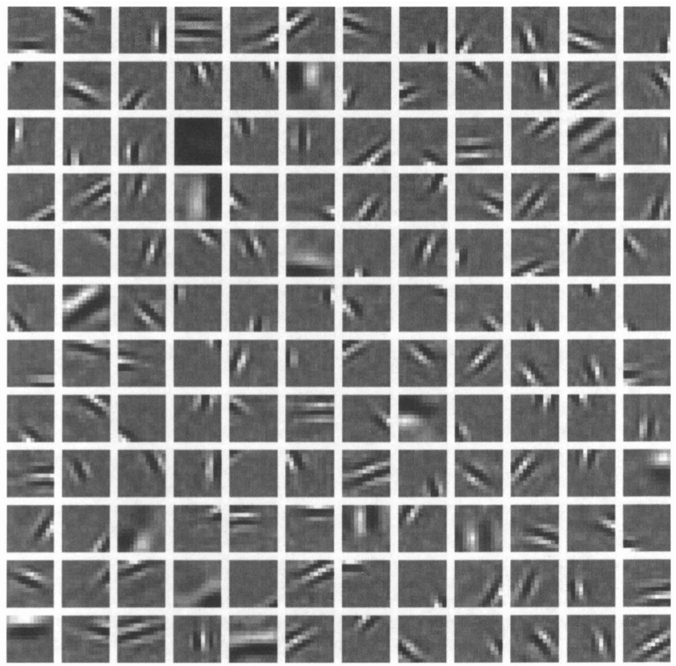
When ICA is applied to natural images, the learned bases are Gabor-like edge detectors, similar to early visual receptive fields. This suggests that the independent components of natural images are edges — a finding consistent with the long-standing importance of edge detectors in early computer vision algorithms.

The figure belows features the bases found by ICA with my own implementation.

Foldiak’s Model

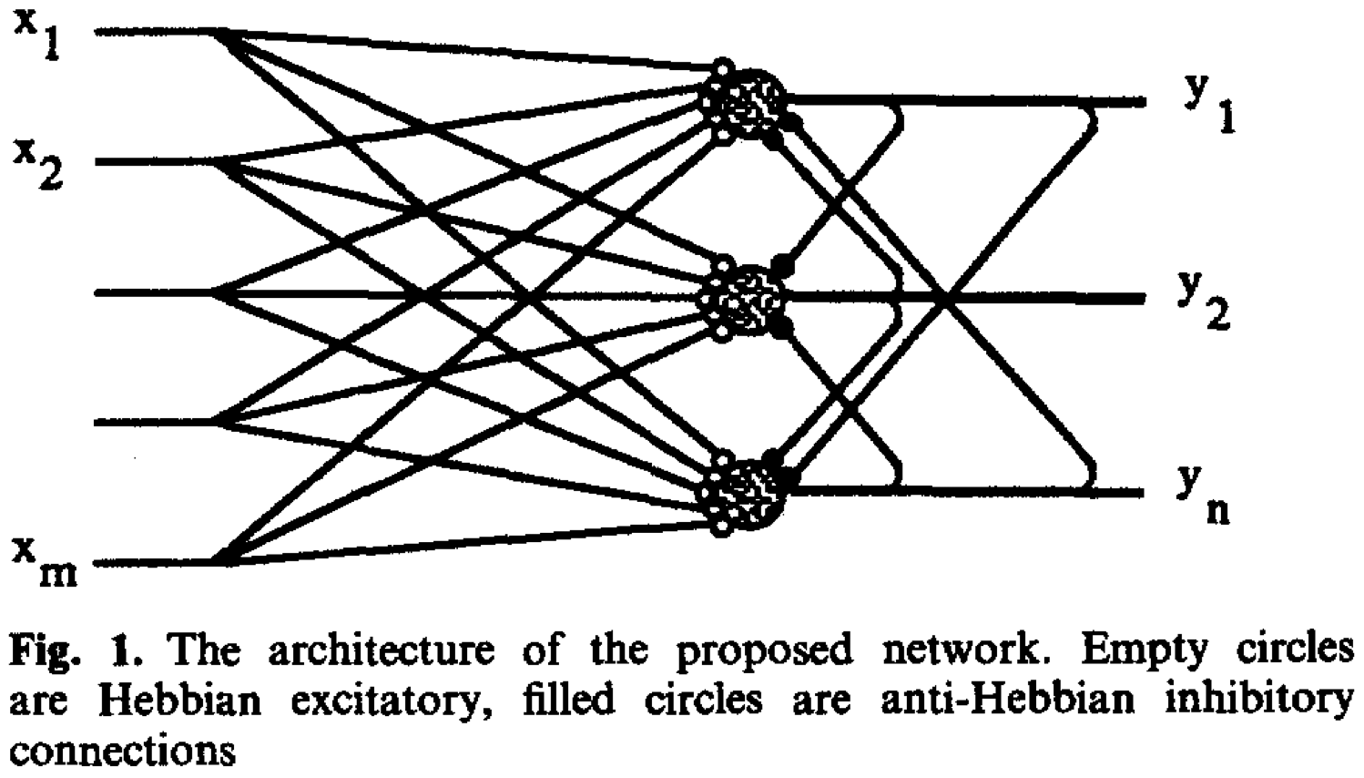
Building on the same redundancy reduction principle, Foldiak (1990) proposed a learning rule combining both Hebbian and anti-Hebbian terms. The model has two layers. The feedforward weight, connecting the input and output layer, is learned by Hebbian rule, which serve as pattern recognition by detecting suspicious coincidences. To avoid units detecting the same patterns, lateral connections within the same layer are introduced, whose weights are learned by the anti-Hebbian rules. Whenever two units in the layer are active simultaneously, the connection between them becomes more inhibitory. These two terms, together with a threshold modification term, ensure that the activation is sparse.

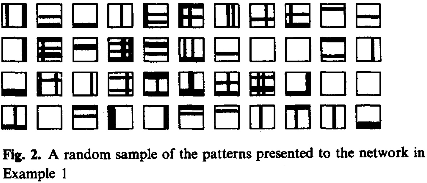
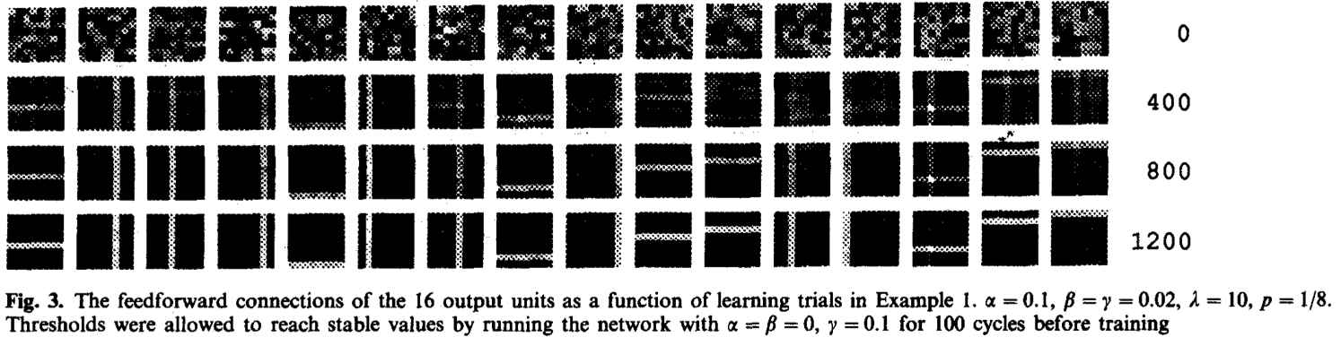
When applied to images of horizontal and vertical stripes, Foldiak’s model learns line segments resembling edge detectors.

Inputs:

Cell visualization:

Sparse Coding

In their landmark 1996 Nature paper, Olshausen and Field showed that minimizing reconstruction error while enforcing a sparsity constraint on the coefficients $a$ allows the following generative model to learn bases resembling edge detectors.

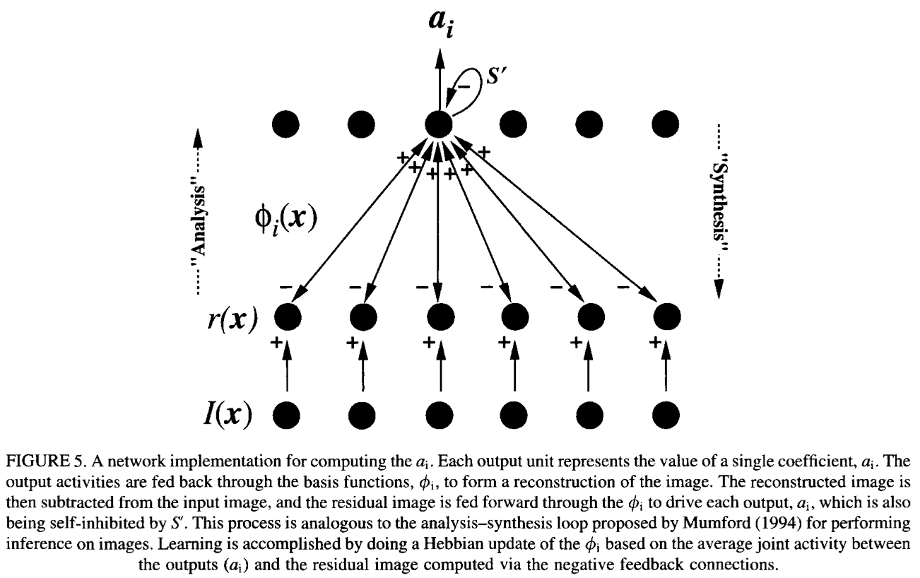
The update rule for the basis functions $\phi$ is Hebbian in nature:

$$\Delta \phi = a \cdot (I - \tilde{I})$$

The resulting filters are Gabor-like, and the authors note that this outcome is likely not unique to their model — other frameworks under similar constraints would probably converge to similar representations.

Backpropagation

Independently invented and reinvented by multiple researchers, and subsequently popularized by Rumelhart and Hinton in 1986, the backpropagation algorithm became the dominant method for training artificial neural networks. Although backprop is widely regarded as biologically implausible, Machine learning and AI researchers are less concerned because they focus more on benchmark performance.

What makes backprop relevant here is that deep neural networks trained with it also develop early-vision-like selective cells without ever being told to. Jarrett et al.¹⁴ showed that randomly initialized CNNs, when optimized via backprop to find their preferred inputs, seek out stripe-like patterns.

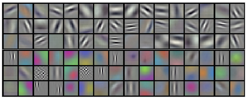
AlexNet, when trained with supervised learning on ImageNet, develops Gabor-like filters in its first layer.

Backprop Alternatives?

Given the wildly success of the biologically-implausibility backprop in AI, a relevant question is, are there learning rules that are both biologically grounded and competitive? There is no clean answer. Below are two serious attempts.

Contrastive Hebbian Learning: Hinton’s Relentless Pruisuit

The Boltzmann machine (Hinton & Sejnowski, 1986) is an early attempt from Hinton. A two-layer model with symmetric weights, its learning rule has the form:

$$ \Delta w_{ij} = \epsilon (p_{ij} - p’_{ij})$$

The first is a Hebbian term: the visible units are clamped to real data and the network is allowed to settle to equilibrium. The second is an anti-Hebbian term: the units are free to evolve from a random initialization. Together, these terms push the model’s internal distribution — its “world model” — toward matching the true distribution of the environment.

This contrastive structure became a recurring motif in Hinton’s career, threading through deep Boltzmann machines, variational inference, contrastive learning, and culminating in the forward-forward algorithm — his most explicit attempt yet to displace backprop, which sees limited adoptation in a performance-driven research atmosphere.

Complex Cells and Predictive Coding

A separate thread comes from predictive coding¹⁵, a framework with deep roots in both theoretical neuroscience and signal processing. The core idea is that higher layers send top-down predictions to lower layers, and lower layers propagate prediction errors upward.

This framework offers a good explanation of the hypercomplex cell behavior such as end-stopping. Moreover, it has been shown that under certain conditions predictive coding and backpropagation are mathematically equivalent.

Final Words

The convergence of features learned by Hebbian rules and backpropagation in the visual domain points to a profound connection between neuroscience and AI — two fields long united by a common ambition: understanding and reverse-engineering the brain and mind. Yet modern AI has steadily drifted from its biological roots, favoring brute-force engineering over principled inspiration. Scaling current architectures can take us remarkably far, but the landscape of ideas is growing repetitive, energy costs are spiraling, and fundamental challenges — like efficient skill acquisition from few samples — remain stubbornly unsolved. My intuition is that the next breakthough will likely be achieved by looking backward: toward neuroscience, cognitive psychology, and the still-unresolved mysteries of biological minds.