Nearly four decades ago, Geoffrey Hinton published “Learning Distributed Representations of Concepts” (1986), with key findings also appearing in his influential Nature paper, “Learning Representations by Back-Propagating Errors”. These papers are historically famous for popularizing backpropagation, but this post focuses on two of their lesser-known aspects: an early example of what we’d now recognize as language modeling, and pioneering work in mechanistic interpretation.
What made Hinton’s work particularly prescient was not just the learning algorithm itself, but the experimental framework he chose to demonstrate it. Hinton’s task was elegant: predict family relationships across two isomorphic family trees—a challenge that essentially amounts to what we’d now call a (tiny) language model. For instance, given “Colin has-father James” and “James has-wife Victoria”, the network learns to predict the answer to “Colin has-mother ?”. Beyond the task itself, Hinton provided detailed visualizations and interpretations of the network’s internal representations—an early foray into what we now call mechanistic interpretability.
Academia naturally gravitates toward the latest research, but classic papers remain treasure troves of ideas, intuitions, and hands-on learning opportunities. This post focuses on Hinton’s family-tree experiments, first reproducing Hinton’s original MLP results, then extending the analysis to modern transformer models.
Background: How Are Concepts Encoded in Neural Networks?
In 1986, two competing paradigms dominated thinking about concept representation in neural networks:
Localist representation: Each concept is assigned to a single dedicated node.
Distributed representation: A concept is encoded through the joint activation of many nodes.
Hinton was a vocal proponent of distributed representations. He even dedicated an entire book chapter to demonstrating that distributed representations not only solve the binding problem inherent in localist representations, but also encode concepts far more efficiently. In this paper, however, Hinton identified a critical limitation of distributed representations as they were typically implemented: concepts were encoded as fixed activation patterns, invariant to context or role.
Consider John as an example. At work, John is an AI researcher—reading papers, training models, debugging code. At home, he’s a father of three—telling bedtime stories, playing with his kids, helping with homework. If a network encodes John with a single fixed activation pattern, it cannot capture how his identity shifts across these different contexts.
To address this limitation, Hinton proposed an architecture where concepts and their roles are encoded separately by distinct groups of neurons. He trained a five-layer network using gradient descent, then visualized and interpreted its learned weights—revealing how concepts were encoded and what individual neurons had specialized to represent.
Family Tree Prediction Task
To motivate the idea of role-specific nodes, Hinton introduced the family tree prediction task:
The setup involves two isomorphic family trees—one with English names, one with Italian names. “Isomorphic” means the trees share identical structure, but with different individuals. For example, in the figure below, Christopher is married to Penelope, and they have two children: Arthur and Victoria. Each tree contains 12 individuals, for a total of 24 unique names across both trees.
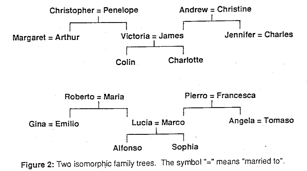
The task considers 12 types of relationships: father, mother, husband, wife, son, daughter, uncle, aunt, brother, sister, nephew, and niece. Across both trees, there are 104 relationship instances—triplets like (Margaret, has-father, Christopher). Some relationships involve multiple individuals: Colin has two uncles (Arthur and Charles), represented as (Colin, has-uncle, (Arthur, Charles)).
The network’s goal is to predict the third element given the first two. For instance, given (Margaret, has-father, ?), the model should output Christopher.
Network Architecture
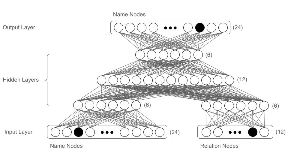
Hinton’s architecture is a five-layer MLP with a distinctive structure:
The input layer contains 36 nodes: 24 nodes encode individual names, and 12 nodes encode relationship types.
The first hidden layer splits into two groups of 6 nodes each. One group connects exclusively to the name inputs, the other exclusively to the relationship inputs. This separation enables the network to encode concepts (individuals) and roles (relationships) independently.
The second and third hidden layers contain 12 nodes and 6 nodes respectively, both fully connected.
The output layer mirrors the input’s name representation with 24 nodes, one per individual.
All layers use sigmoid activation functions. The network architecture is visualized below.
Network Visualization and Interpretation
Many of the learned weights prove to be interpretable. Hinton visualizes this by examining the first hidden layer’s weights—specifically, the 6 nodes connected to name inputs—across all 24 individuals.
In the figure below, each colored line corresponds to one hidden node. Square size indicates activation strength, while color indicates sign: white for positive activation, black for negative.
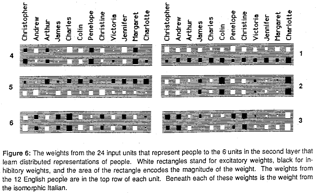
Due to space constraints, the paper displays only English names. The corresponding Italian names from the isomorphic tree appear as the second line in each visualization.
The visualization reveals several striking patterns in what the network learns: Nodes 1 and 5 both distinguish between English and Italian names—Node 1 activates for English, Node 5 for Italian. While this seems redundant, it’s a natural outcome when networks freely learn any features that reduce loss. Weight decay often encourages such redundancy.
The architecture compresses the 24-dimensional one-hot input into 6 dimensions, forcing the network to retain only essential information. Given the trees’ isomorphic structure, the most efficient compression encodes tree origin in a single bit. Remarkably, without any explicit knowledge of input semantics, the network discovers this property autonomously—using just one or two nodes to indicate tree membership.
In other nodes, English names and their Italian counterparts produce nearly identical activations, confirming the symmetry between trees.
Node 2 encodes generational depth: third-generation members like Charlotte and Colin show strong negative activations.
Node 6 captures family branch information. All individuals on the right half of the tree trigger negative activations—a consistent and intriguing pattern.
Notably, gender isn’t encoded by name input nodes. This makes sense: the task doesn’t require gender to determine relationships. Knowing Colin’s gender, for instance, isn’t necessary to identify his father.
Gender is instead encoded in the the relation input nodes. Node 5 (middle figure, bottom row) clearly encodes gender—male relations produce negative activations, female relations positive ones.
Node 3 correlates strongly with generational hierarchy: positive for senior relations, negative for younger ones.
Reproduction
I reproduced Hinton’s family tree experiment in PyTorch (code here). Modern deep learning offers countless conveniences unavailable in 1986—optimizers like Adam, automated differentiation, standardized frameworks. Rather than strictly replicate Hinton’s original setup, my goal was to optimize network performance on the test set using contemporary best practices.
Reproducibility: The Ghost That Haunts My Mind
When you publish a result, you expect it to generalize. How can one claim scientific rigor if peers cannot reproduce their findings? Yet reproducibility remains frustratingly elusive. It manifests on at least two levels: same-machine reproducibility and cross-machine reproducibility.
Same-machine reproducibility can typically be achieved by fixing random seeds and locking package versions. Cross-machine reproducibility is far more elusive.
I train exclusively on CPUs with single-threaded data loading to eliminate parallelism as a factor. Yet discrepancies persist. The culprit? Different CPUs use different math acceleration libraries (MKL, OpenBLAS, etc.), each with subtle implementation differences. These low-level variations are enough to break reproducibility.
As a quick example, I ran the following code on both my laptop (MacBook Air M4, 2025) and desktop (Ubuntu 24.04.1 LTS, Intel i7-12700K), using identical Python environments managed by uv:
import torch
torch.manual_seed(42)
x = torch.randn(10000, 10000)
y = torch.mm(x, x.t())
print(y.sum().item())
The results: 99229240.0 on Mac, 99229296.0 on Ubuntu—a relative difference of 5.64e-7. While negligible in most contexts, this is enough to cause accuracy metrics to diverge.
The reproducibility rabbit hole runs deep. I remember reading as a child about scientists who took their own lives when their findings couldn’t be replicated. Perhaps that’s when this obsession with reproducibility took root in me. Whether it’s a necessary discipline or an unnecessary burden, I honestly don’t know.
MLP Model
Given the small dataset size, the model is highly sensitive to weight initialization. To account for this, I evaluated test performance across 50 different random seeds. I also randomly shuffled the train/test split for each seed to avoid overfitting to any particular split.
Since Colin has two uncles, family tree prediction is a multi-label classification problem. I used MultilabelAccuracy as the primary metric, with outputs above 0.5 considered positive predictions. Accuracy equals 1 only when all labels are predicted correctly (exact match).
My 5-layer MLP architecture follows: 24+12 → 6+6 → 6 → 12 → 32 → 24. It achieves an average accuracy of 0.725, with 20 of 50 runs reaching perfect accuracy (4/4 correct on the test set).
Below is a summary of techniques tested, categorized by their impact on accuracy. Improvements:
Adam/AdamW: Adam converges far faster than SGD. Weight decay (AdamW) improves generalization. All runs achieved 100% training accuracy, so the challenge is purely reducing overfitting.
Batch normalization: Accelerates training convergence.
Deeper architectures: Structured expansion/reduction (especially 2× factors) proved crucial for generalization.
Learning rate warm-up: Consistently improved test performance by small margins.
Gradient clipping: Another universal technique that slightly boosts test accuracy.
Hard labels: Counterintuitively, hard labels (1.1, -0.1 instead of 1.0, 0.0) improve test accuracy. Since MSE loss is satisfied when outputs reach 0 or 1, larger-margin labels force the model to better separate positive and negative signals.
Hyperparameter tuning: Learning rate and epoch count require careful tuning. Grid search would help but wasn’t pursued here.
Bug fixes: Setting bias=True before batch norm layers is a subtle but critical mistake to avoid.
Degradations:
ReLU activation: Despite ReLU’s success in deep learning, sigmoid substantially outperforms it for this task.
Custom weight initialization: Xavier initialization and uniform ranges like (-0.3, 0.3), (-0.1, 0.1), (-0.5, 0.5) all underperformed PyTorch’s default initialization.
Neutral (No Clear Impact):
- Soft labels
- Multi-label loss functions
Transformer architecture
The family tree prediction problem maps naturally onto language modeling: predict the next token given previous tokens. While feeding all known triplets into a modern LLM (GPT-4, Claude, Gemini) would likely yield high accuracy, this experiment takes a different approach. I trained a small decoder-only transformer from scratch to better match the MLP baseline setting.
I borrowed a lot of code from nano-GPT. An initial version gets 0.35 average accuracy. Not bad for the first-try, but I have higher expectations from transformers. Most training tricks for MLP also apply to transformer: learning rate warmup, gradient clipping, AdamW, and learning rate/epochs tweaking, etc. When I try to tweak the network architecture, specially trying out new non-linearity, normalization, and other hyperparameters like expansion factor, all trials fail really badly. The transformers are not popular without a reason. These network components are really put together in an “optimal” way. Changing anything inside would break the whole system. I then restrict myself to only change the following hyperparameters: n_layer,n_head,n_embd,and dropout.
I explored the hyperparameter space using both Weights & Biases’ Bayesian optimization and a custom grid search script. The best configuration found was:
n_layer: int = 2
n_head: int = 14
n_embd: int = 112
dropout: float = 0.2
The final accuracy number is 0.715, comparable to the MLP model.
Encoder Transformer
For the classification formulation, we could use an encoder-only transformer (BERT-style). The modifications are straightforward: remove the attention mask, prepend a token to the input, and compare its output embedding to the target.
However, I only achieved ~0.4 accuracy with the encoder model. The key difference, I suspect, is that the decoder model computes loss on both the second input token and the final output, while the encoder model only computes loss on the output. The additional training signal from the second input position—though noisy—appears to help the model learn more effectively.
Visualizations
I visualized the first-layer weights of the trained MLP model for both name and relationship inputs. The plot below shows the name node embeddings using random seed 0, where the model achieved 3/4 correct predictions. Additional visualizations can be found in the GitHub repo.
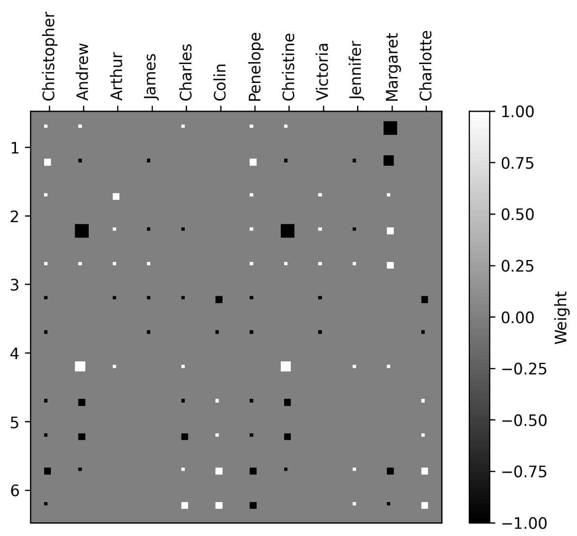
The visualizations reveal two notable patterns:
Nodes 3 and 4 specialize in distinguishing English from Italian names. Nodes 5 and 6 encode generational depth, with older generations producing increasingly negative activations.
These patterns align with Hinton’s original findings, though the separation in my results is less distinct.
Final Thoughts
Hinton’s paper, while groundbreaking, can be difficult to parse due to its age and writing style. I hope this blog provides a more accessible entry point, though I encourage you to read the original—you may catch nuances I overlooked.
I find deep satisfaction in reproducing classic experiments. These small-scale, carefully designed setups provide ideal testbeds for experimenting with learning rates, optimizers, architectures, and training techniques. They demonstrate how thoughtful experimental design can yield profound insights into learning systems. My implementation prioritizes clarity over polish—feel free to build on it and explore methods that might improve test accuracy.
Visualizing first-layer weights remains common practice in computer vision, revealing features like edge detectors or color channels in CNNs. Deeper layers, however, resist interpretation due to increasing complexity and non-linearity. For those, techniques like maximally-activating inputs, gradient-based input modifications (combined with priors for natural-looking images), or sparse autoencoders (in transformers) prove more effective.
Perhaps the most striking discovery from this reproduction: many “standard” training techniques—momentum, label smoothing, learning rate warmup, stochastic gradient descent—were already proposed and explored in the 1980s. We take these tools for granted today, but Hinton’s early focus on training methodology laid the groundwork for neural networks’ eventual mainstream adoption, decades before the deep learning revolution.
Role-Specific Representations
The family tree experiment was motivated by the concept of role-specific representations. Hinton argued that to truly understand relationships, networks must encode not just entity identity but also contextual role. He introduced grouped neurons—separate subsets independently encoding identity and role.
This concept presages his later work on capsule networks, which aim to disentangle object properties from spatial relationships. In my view, modern LLMs achieve a similar effect through attention mechanisms, which dynamically and flexibly associate entities with their contextual roles.
Inductive Bias
Different architectures embody different inductive biases, making them suited to different tasks. In a later paper (Learning Distributed Representations of Concepts Using Linear Relational Embedding), Hinton acknowledges that MLPs struggle to find optimal solutions for this task and proposes Linear Relational Embedding instead. The core idea: represent concepts as vectors, binary relations as matrices, and relation application as matrix-vector multiplication that approximates the related concept. Representations are learned by maximizing a discriminative objective via gradient ascent.
Is It Worth the Effort?
You might wonder why invest so much effort in a toy experiment few care about today. I’m reminded of the possibly apocryphal story of Leonardo da Vinci’s egg drawings:
When young Leonardo apprenticed under Andrea del Verrocchio, his master made him draw hundreds of eggs from different angles to teach him about form, light, and shadow. Verrocchio told him that no two eggs are identical and each viewing angle reveals something new.
Whether true or not, the story captures something essential about both artistic training and model development: fundamental intuitions emerge through repeated engagement with simple problems.