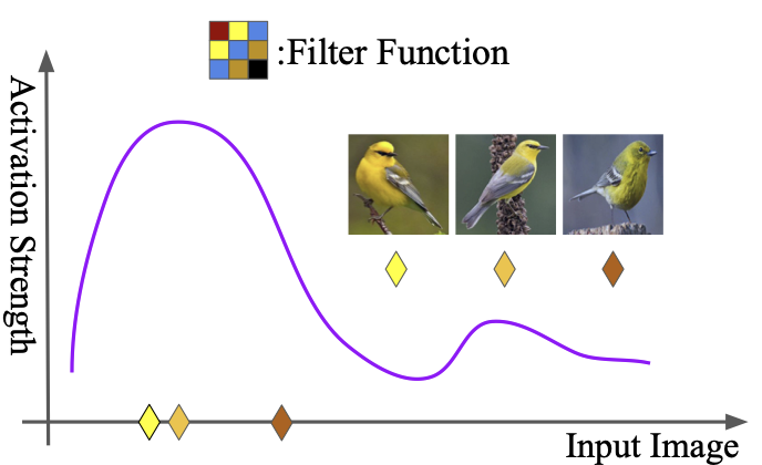
If we display the maximally activating images of a neuron in a randomly initialized autoencoder, a surprising phenomenon emerges: a network filled with random noise nonetheless contains some neurons that are sensitive to specific features.
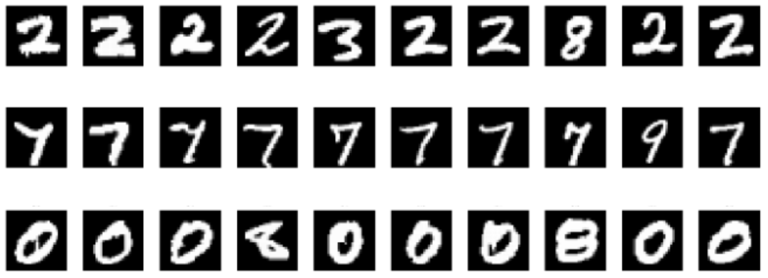
This raises a question: is this a bug in the interpretability method itself, or does it reveal some essential feature of the neural network?
Distributed representation
Due to the property of distributed coding in neural networks, the natural basis (visualizing individual neurons) may not be the best way for understand. This is analogous to thermodynamics, where the trajectory of a single atom may be random and meaningless, yet the statistical properties of countless atoms can be characterized by macroscopic quantities like temperature and pressure.
Szegedy, et al. [1] discovered early on that randomly weighting the hidden layer neurons of a trained neural network still yields units with strong interpretability.
More unsettling is that this property holds even in randomly initialized networks.
Sparse Autoencoders (SAE)
To decompose these distributed features, the recently popular SAE (Sparse Autoencoders) method attempts to map network activations into a higher-dimensional sparse space. Viewed through the lens of Dictionary Learning, SAE seeks to solve:
$$x \approx D\alpha$$
where $x$ is the activation vector, $D$ is the learned dictionary, and $\alpha$ is a high-dimensional sparse vector.
- If $\alpha$ is 1-hot sparse, SAE degenerates into Vector Quantization — finding the nearest cluster center.
- Otherwise, SAE approximates a non-orthogonal, nonlinear version of PCA.
The core assumption of SAE is that by enforcing sparsity, we can find a set of basis vectors that are more “natural” and better aligned with human concepts than individual neurons.
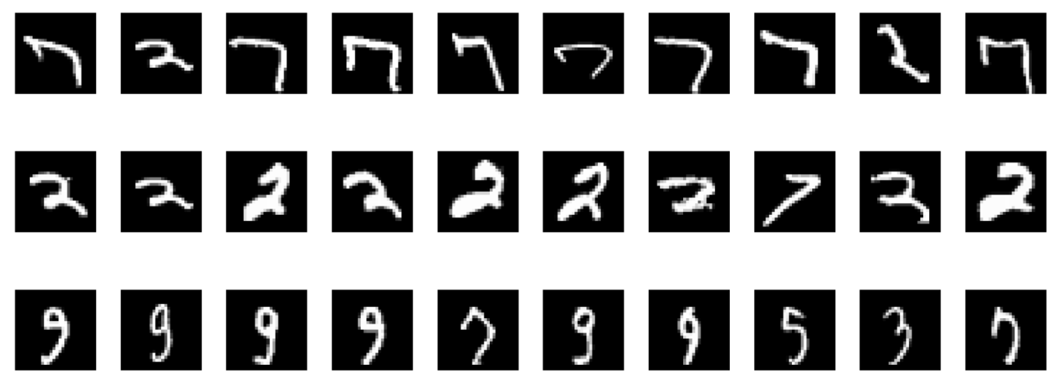
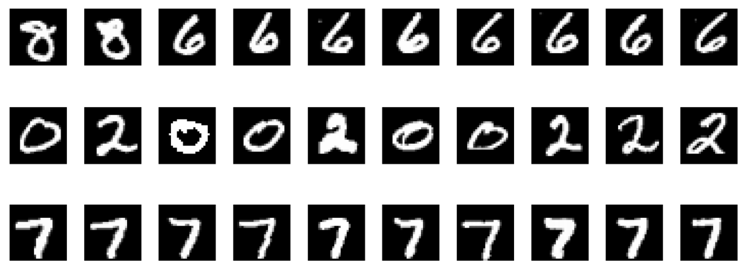
Yet the strange thing still happens: even running SAE on a randomly initialized network, we can still find a large number of “interpretable” units.
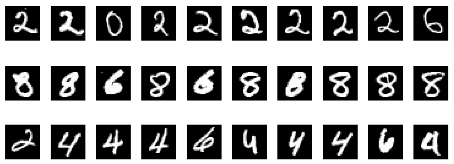
From the examples above, we can conclude that randomly initialized neural networks contain local structures sensitive to certain features. Indeed, several recent papers [2, 3] confirm this: randomly initialized BERT or Transformer models can also be interpreted as exhibiting syntactic or semantic features. An earlier important paper by Adebayo et al. [9] similarly found that for randomly initialized CNNs or networks trained on randomized labels, the vast majority of interpretability methods can still find interpretable features such as edge detectors. People tend to see these as evidences for the inadequacies of the interpretation tools, but are there any perspectives worth discussion?
Network Properties: Architecture as Prior?
The interpretability exhibited by random networks is not necessarily a failure of the explanation tools — it may profoundly reveal the inductive bias embedded in deep neural network architectures: the network architecture itself encodes a tremendous amount of knowledge.
In computer vision, Jarrett et al. [4] showed that the structure of CNNs itself tends to capture the statistical regularities of images (such as smoothness and edges), to the point where a fixed, randomly initialized network with just one learnable linear layer can achieve classification results comparable to supervised learning. [7, 8] similarly noted this phenomenon and applied it to rapid neural architecture screening. Deep Image Prior [5] went further, proposing that even with only a single training image, a randomly initialized CNN can serve as an effective image prior for tasks like denoising or super-resolution.
In computational neuroscience, Rosenblatt’s perceptron model [12] was originally a three-layer neural network with a randomly initialized input layer and a trainable output layer. Studies on the Drosophila brain have found that one layer appears to use random connectivity. Random connectivity — rather than backpropagation — not only has biological grounding but biological meaning. Rosenblatt [12] proved its effectiveness on linearly separable data. Reservoir Computing [11] with a fixed, randomly initialized RNN and a trained final linear readout layer can handle complex temporal/sequential tasks.
In traditional statistical machine learning: Rahimi and Recht [6] proposed that mapping high-dimensional features to a lower-dimensional space via specific random rules enables large-scale SVM using the kernel trick. The Viola-Jones detector achieves solid detection results by boosting weak classifiers trained on random features. The Johnson-Lindenstrauss Lemma shows that random projections from high-dimensional to low-dimensional spaces preserve data structure (pairwise distances). Cover’s Theorem proves that high-dimensional spaces are more likely to produce linearly separable features. In compressed sensing it is shown that a random linear project and L1 constraint can yield a sparse code for the input with a high probability.
The Lottery Ticket Hypothesis
Everything above seems to suggest that random mappings can to a large extent preserve structure in the data. This has a connection to the Lottery Ticket Hypothesis: within a randomly initialized, over-parameterized network, there exists “winning” subnetworks that got luckily initialized to a favorable position to solve the problem alone, while the remaining weights cancel each other out without degradation. This hypothesis may serve as one theoretical support for the effectiveness of architectural scaling.
Examining Interpretability Methods
We’ll now examine the interpretability methods themselves.
We must first recognize that what we are studying is a function — a mapping from inputs to outputs.
Traditional wisdom holds that this function is strongly non-convex, possessing multiple local extrema.
Are Neural Networks Non-convex?
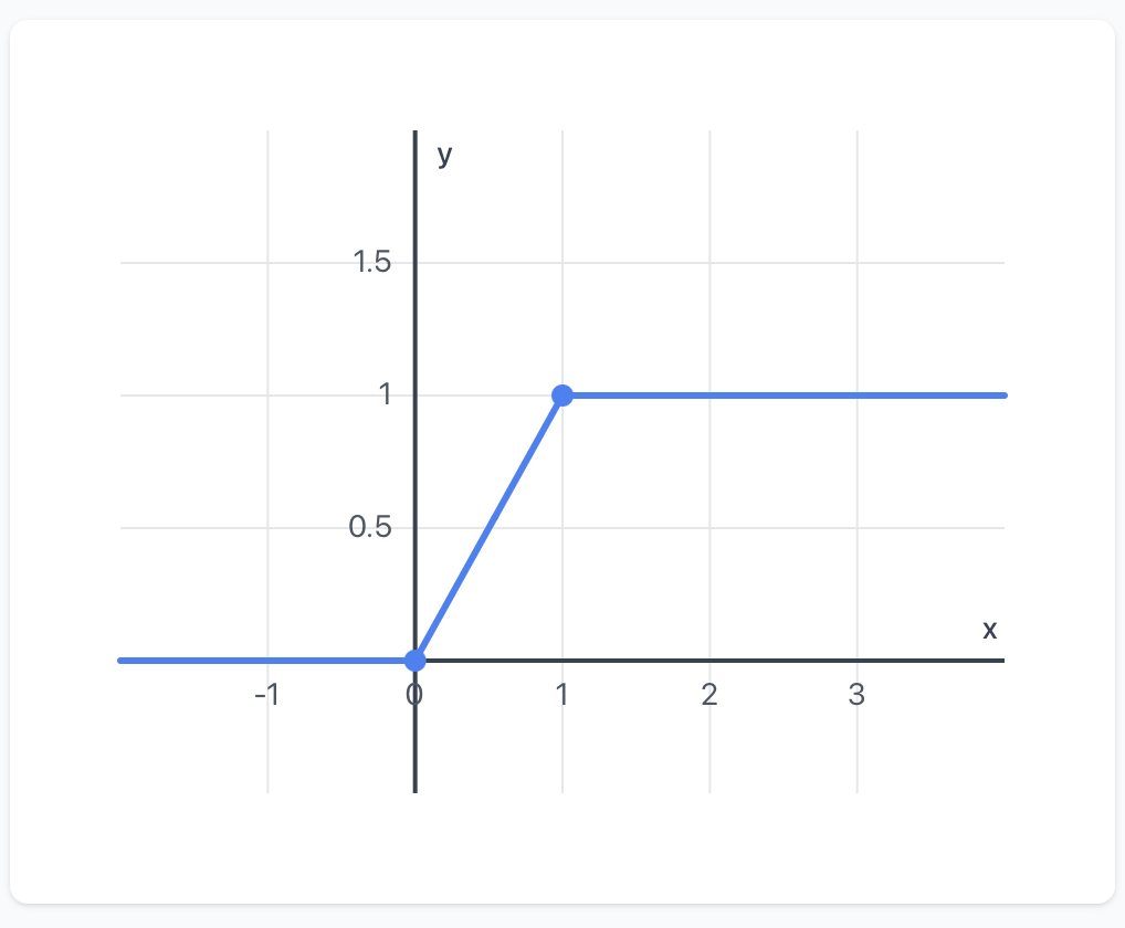
It is not difficult to construct a network whose final-layer function can be expressed as: $$y = \text{max}(\text{max}(x, 0) - \text{max}(x-1, 0), 0)$$
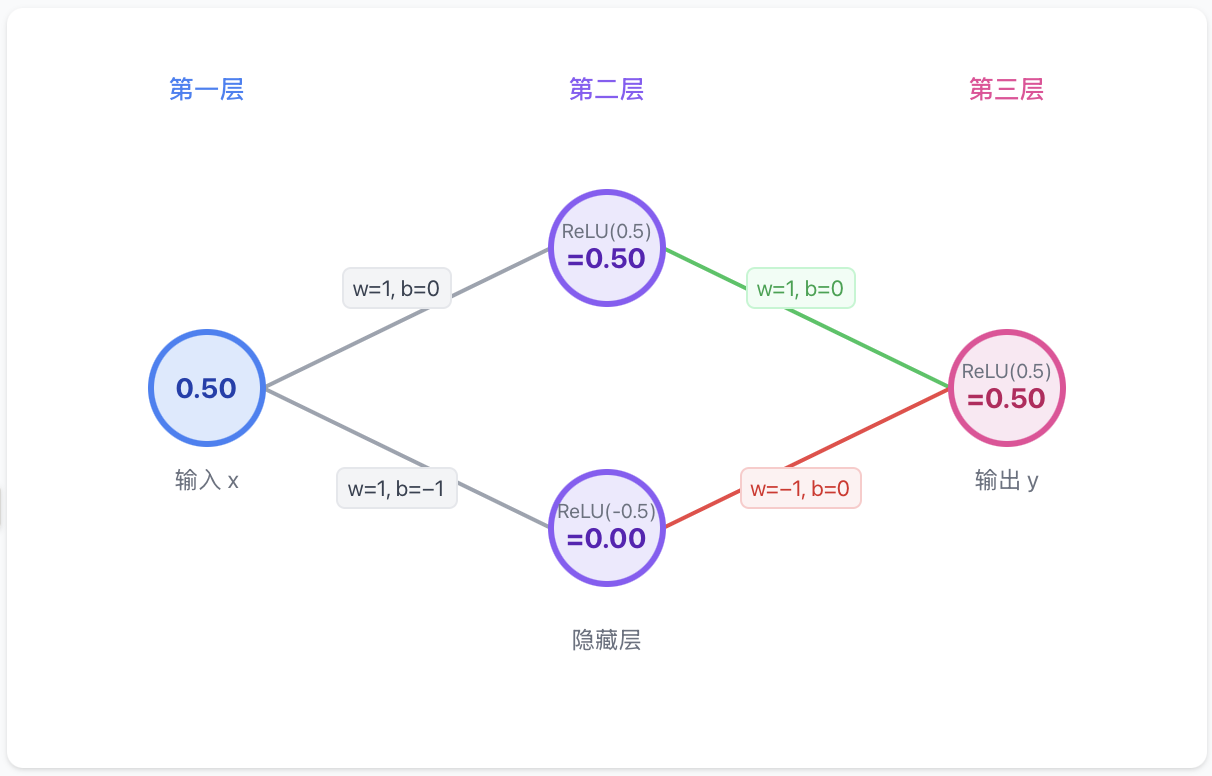
This is a non-convex, non-concave function as shown below.
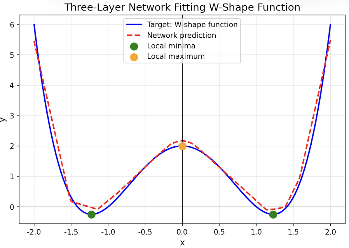
We can even construct a three-layer neural network with two local minima, achieved by fitting: $$y = x^4 - 2x^2 + 0.5$$
But in Practice…
Just because a network can be non-convex doesn’t mean it will be. For a randomly initialized network, contrary to intuition, most loss curves are quasi-convex/concave.
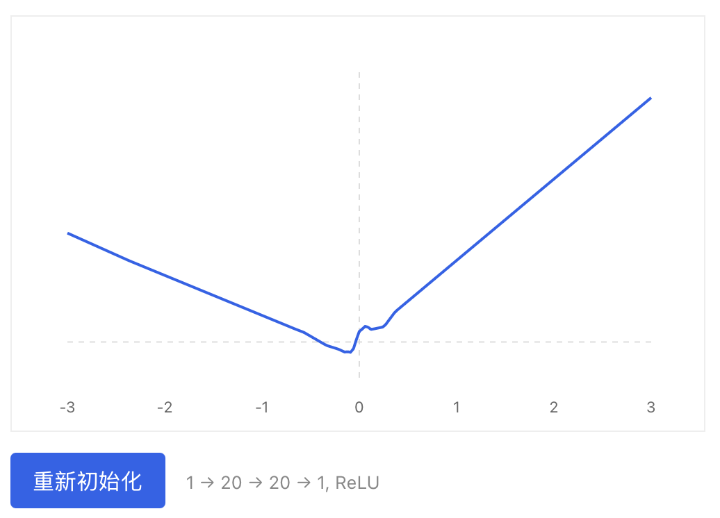
A small bias appears to be key to quasi-convexity — notably, Xavier initialization sets biases to zero, which greatly increases convexity.
Dauphin et al. [10] shows that in high-dimensional spaces, the loss landscape may have far fewer local minima than imagined, with saddle points being more common. The intuition is that for a true local minimum, all directions must curve upward — a low-probability event in high dimensions. There are always smooth directions that allow stochastic gradient descent to escape local minima. Limitations of Maximum Activation Visualization
Here we discuss the limitations of the maximally activated images as a faithful way of understanding neuron activation patterns. We can see this by the following arguments.
If the function has many local extrema: characterizing a non-convex function by its maximally activating input is inherently inaccurate. We cannot guarantee that the maximally activating input in the dataset corresponds to the true maximum, nor can we establish whether the input data lies within the same basin or is randomly distributed across different basins.
If the function does not have many local extrema: we know the function has certain properties — continuity, and even Lipschitz continuity (a small perturbation in input produces only a small perturbation in output). If the input data is sufficiently dense, we can sample data similar to the maximum point in its vicinity, all of which will strongly activate the neuron. Using this to claim the network has learned useful features is insufficient — it is actually a byproduct of data density and relative function continuity, not direct evidence that the network has learned meaningful features. In other words, maximally activated samples only work if we assume the function is convex and the inputs are diverse enough to cover the extreme points.
A Better Approach
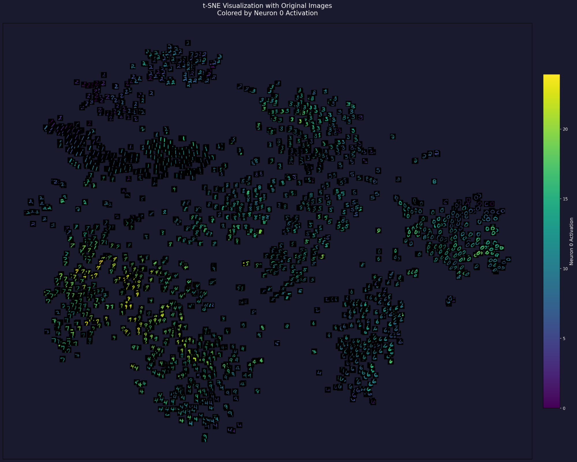
A crucial step is to fully characterize the activation distribution, not just the peak input. One simple approach is to overlay a heatmap on t-SNE to obtain global activation information. This visualization provides a much richer landscape than maximally activating inputs alone.
Conclusion
A fundamental question is: what is the purpose of interpretability? For me, it should help us understand networks in order to design better ones. Like a good theory of learning, it should not only explain known facts, but also needs to predict new capabilities. From this perspective, the problem with mainstream interpretability methods is that they do not create new knowledge — they are used only to passively explain existing knowledge. As new network architectures continuously iterate, interpretability methods rapidly become obsolete. The same applies to some of the theories for deep learning: a theory developed for CNNs may quickly become irrelevant with the advent of Transformers.
The fascinating and puzzling properties exhibited by randomly initialized networks represent a genuinely interesting research problem. Perhaps deeper understanding lies here: high-dimensional spaces contain many phenomena that are difficult to comprehend from a low-dimensional perspective. Learning to better understand high-dimensional spaces is likely the key to understanding both artificial and biological neural networks — and may be a more promising direction than interpretability methods alone.
References
[1] Christian Szegedy, Wojciech Zaremba, Ilya Sutskever, Joan Bruna, Dumitru Erhan, Ian Goodfellow, Rob Fergus, Intriguing properties of neural networks.
[2] Thomas Heap, Tim Lawson, Lucy Farnik, Laurence Aitchison, Sparse Autoencoders Can Interpret Randomly Initialized Transformers
[3] Maxime Méloux, Giada Dirupo, François Portet, Maxime Peyrard, The Dead Salmons of AI Interpretability
[4] Kevin Jarrett, Koray Kavukcuoglu, Marc’Aurelio Ranzato, Yann LeCun, What is the Best Multi-Stage Architecture for Object Recognition?
[5] Dmitry Ulyanov, Andrea Vedaldi, Victor Lempitsky, Deep Image Prior
[6] Ali Rahimi, Benjamin Recht, Random Features for Large-Scale Kernel Machines
[7] Nicolas Pinto, David Doukhan, James J. DiCarlo, David D. Cox, A high-throughput screening approach to discovering good forms of biologically inspired visual representation
[8] Andrew M. Saxe, Pang Wei Koh, Zhenghao Chen, Maneesh Bhand, Bipin Suresh, and Andrew Y. Ng, On Random Weights and Unsupervised Feature Learning
[9] Julius Adebayo, Justin Gilmer, Michael Muelly, Ian Goodfellow, Moritz Hardt, Been Kim, Sanity Checks for Saliency Maps
[10] Yann Dauphin, Razvan Pascanu, Caglar Gulcehre, Kyunghyun Cho, Surya Ganguli, Yoshua Bengio, Identifying and attacking the saddle point problem in high-dimensional non-convex optimization
[11] Herbert Jaeger, The ”echo state” approach to analysing and training recurrent neural networks.
[12] F. Rosenblatt, The perceptron: A probabilistic model for information storage and organization in the brain.